Python Refresher for DSA

What You Will Learn in This Blog
Python Built-in Data Types for DSA
The Collections Module
List Comprehensions
Important Built-in Functions for DSA
Sorting in Python
String Operations
heapq – The Built-in Min Heap
Common Python Patterns in DSA
Summary
Key Takeaways
Next Steps

What You Will Learn in This Blog

The Python built-in data types you will use constantly in DSA
How lists, dictionaries, sets, and tuples work and when to use each
Important Python built-in functions and their complexities
The collections module – deque, defaultdict, Counter
List comprehensions and when to use them
Common Python patterns that appear repeatedly in DSA problems

This is not a complete Python tutorial. It covers exactly what you need to follow the rest of this guide comfortably. If you are already confident with all of the above, you can skim this and move on.

A note on time complexity notation

Throughout this blog you will see notations like O(1), O(n), and O(n log n) next to operations. These describe how the time or memory an operation takes grows as the input gets larger. They are covered in full detail in the next blog – Complexity Analysis. For now, here is just enough to follow along:

Notation	Plain English
O(1)	Takes the same time regardless of input size – constant
O(n)	Time grows linearly with input size
O(n log n)	Slightly worse than linear – typical of good sorting algorithms
O(n^2)	Time grows quadratically – usually something to avoid for large inputs

You do not need to deeply understand these yet. Just use the table as a reference as you read. Everything will become clear in the next blog.

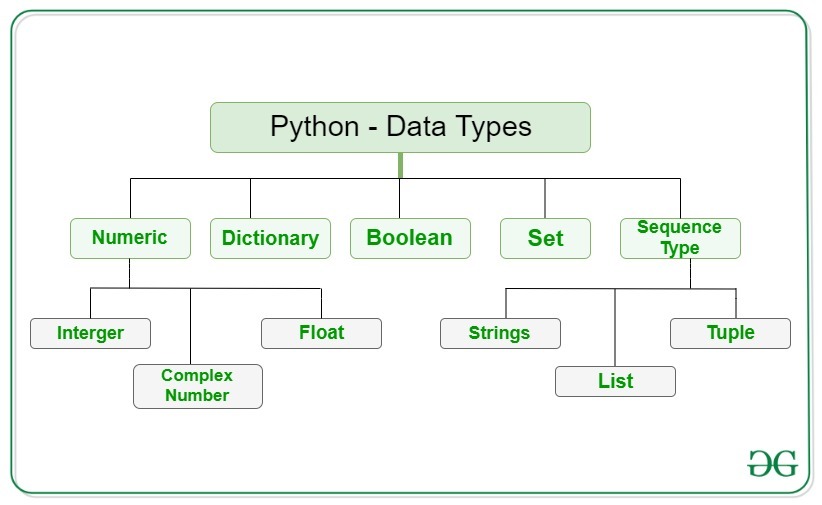
Python Built-in Data Types for DSA

Python gives you several built-in data types that map directly to fundamental data structures. Understanding how they work under the hood will make your complexity analysis much more accurate later.

Python data structures overview

Lists

A Python list is a dynamic array. It can hold elements of any type, grows automatically when you add to it, and supports indexing.

# Creating a list
numbers = [10, 20, 30, 40, 50]

# Indexing -- accessing elements by position
print(numbers[0])   # 10  -- first element
print(numbers[-1])  # 50  -- last element (negative indexing counts from the end)
print(numbers[-2])  # 40  -- second from last

Slicing

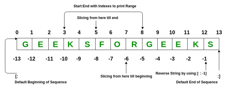
Slicing lets you extract a portion of a list. The syntax is list[start:end:step] where end is exclusive.

Python list slicing diagram

numbers = [10, 20, 30, 40, 50]

print(numbers[1:4])    # [20, 30, 40]  -- index 1 up to but not including index 4
print(numbers[:3])     # [10, 20, 30]  -- from start up to index 3
print(numbers[2:])     # [30, 40, 50]  -- from index 2 to end
print(numbers[::2])    # [10, 30, 50]  -- every second element
print(numbers[::-1])   # [50, 40, 30, 20, 10]  -- reversed list

Common List Operations and Their Time Complexity

Note on complexity notation: You will see terms like O(1), O(n), and O(n log n) in the tables below. These come from Big O notation, which is covered in full detail in the next blog – Complexity Analysis. For now, read them loosely as follows: O(1) means the operation takes the same time regardless of input size, O(n) means the time grows with the size of the input, and O(n log n) means slightly worse than O(n). Once you read the next blog, come back and these tables will make complete sense.

This table is important. Knowing these complexities will directly affect the choices you make when solving problems.

Operation	Example	Time Complexity	Notes
Access by index	`nums[i]`	O(1)	Direct memory access
Append to end	`nums.append(x)`	O(1) amortised	Occasionally O(n) when resizing
Pop from end	`nums.pop()`	O(1)
Insert at position	`nums.insert(i, x)`	O(n)	Shifts all elements after i
Delete by index	`del nums[i]`	O(n)	Shifts elements
Search for value	`x in nums`	O(n)	Scans the whole list
Get length	`len(nums)`	O(1)	Stored internally
Slice	`nums[i:j]`	O(k)	k is the size of the slice
Sort	`nums.sort()`	O(n log n)	Timsort
Reverse	`nums.reverse()`	O(n)	In-place

nums = [3, 1, 4, 1, 5, 9, 2, 6]

# Append -- O(1) amortised
nums.append(7)
print(nums)  # [3, 1, 4, 1, 5, 9, 2, 6, 7]

# Pop from end -- O(1)
last = nums.pop()
print(last)  # 7

# Insert at index -- O(n) because elements shift
nums.insert(0, 99)
print(nums)  # [99, 3, 1, 4, 1, 5, 9, 2, 6]

# Check membership -- O(n)
print(5 in nums)  # True

# Sort in place -- O(n log n)
nums.sort()
print(nums)  # [1, 1, 2, 3, 4, 5, 6, 9, 99]

# Sort and return a new list -- O(n log n)
sorted_nums = sorted(nums, reverse=True)
print(sorted_nums)  # [99, 9, 6, 5, 4, 3, 2, 1, 1]

Key point: Inserting or deleting at the beginning or middle of a list is O(n) because Python has to shift all elements. This matters a lot when choosing between a list and a deque later.

Dictionaries

A Python dictionary is a hash map. It stores key-value pairs and gives you O(1) average-case lookup, insertion, and deletion by key.

# Creating a dictionary
student = {
    "name": "Alice",
    "age": 22,
    "grade": "A"
}

# Accessing a value by key -- O(1) average
print(student["name"])   # Alice

# Safe access with .get() -- returns None if key not found instead of raising an error
print(student.get("score"))        # None
print(student.get("score", 0))     # 0  -- default value if key not found

# Adding and updating -- O(1) average
student["score"] = 95
student["age"] = 23

# Deleting -- O(1) average
del student["grade"]

# Check if a key exists -- O(1) average
print("name" in student)   # True
print("grade" in student)  # False

Iterating Over a Dictionary

scores = {"Alice": 90, "Bob": 85, "Carol": 92}

# Iterate over keys
for name in scores:
    print(name)

# Iterate over values
for score in scores.values():
    print(score)

# Iterate over key-value pairs -- you will use this constantly
for name, score in scores.items():
    print(f"{name}: {score}")

Dictionary Time Complexity

Operation	Time Complexity	Notes
Access by key	O(1) average	O(n) worst case – rare with good hash function
Insert / Update	O(1) average
Delete	O(1) average
Search by key	O(1) average
Iterate	O(n)	n is number of key-value pairs

When to use a dictionary in DSA: Any time you need fast lookup by a key – frequency counting, grouping elements, caching results, mapping one value to another.

Sets

A Python set is a hash set. It stores unique elements and gives you O(1) average-case membership testing, insertion, and deletion.

# Creating a set
visited = {1, 2, 3, 4, 5}

# Add an element -- O(1) average
visited.add(6)

# Remove an element -- O(1) average
visited.remove(3)   # raises KeyError if not found
visited.discard(3)  # safe -- does nothing if not found

# Membership test -- O(1) average  (this is much faster than doing x in list)
print(4 in visited)   # True
print(10 in visited)  # False

# Convert a list to a set to remove duplicates
nums = [1, 2, 2, 3, 3, 3, 4]
unique = set(nums)
print(unique)  # {1, 2, 3, 4}

Set Operations

a = {1, 2, 3, 4}
b = {3, 4, 5, 6}

print(a | b)   # Union:        {1, 2, 3, 4, 5, 6}
print(a & b)   # Intersection: {3, 4}
print(a - b)   # Difference:   {1, 2}
print(a ^ b)   # Symmetric difference: {1, 2, 5, 6} -- elements in one but not both

When to use a set in DSA: Any time you need to track what you have already seen, eliminate duplicates, or check membership quickly.

Tuples

A tuple is an immutable list. Once created, it cannot be changed. You will use tuples in DSA to represent fixed pairs or groups of values – coordinates, edges in a graph, keys in a dictionary.

# Creating a tuple
point = (3, 7)
edge = (0, 1, 5)  # node_from, node_to, weight

# Accessing elements -- same as list
print(point[0])  # 3
print(point[1])  # 7

# Tuples can be used as dictionary keys because they are immutable
distances = {}
distances[(0, 1)] = 5
distances[(1, 2)] = 3

# Tuple unpacking -- very commonly used in DSA
x, y = point
node_from, node_to, weight = edge
print(x, y)  # 3 7

Lists vs Tuples: Use a list when the collection will change. Use a tuple when the values are fixed and you want to use them as a key or want to signal that they should not change.

The Collections Module

Python’s collections module gives you specialised data structures that come up constantly in DSA problems. You do not need to build these from scratch – Python gives them to you.

deque (Double-Ended Queue)

A deque lets you append and pop from both ends in O(1). A regular Python list can only pop from the end efficiently – popping from the front is O(n). Use a deque whenever you need a queue.

from collections import deque

# Create a deque
q = deque()

# Append to right -- O(1)
q.append(1)
q.append(2)
q.append(3)
print(q)  # deque([1, 2, 3])

# Append to left -- O(1)
q.appendleft(0)
print(q)  # deque([0, 1, 2, 3])

# Pop from right -- O(1)
q.pop()
print(q)  # deque([0, 1, 2])

# Pop from left -- O(1)  <-- this is what makes deque better than list for queues
q.popleft()
print(q)  # deque([1, 2])

You will use deque every time you implement BFS (Breadth-First Search).

defaultdict

A defaultdict is a dictionary that automatically creates a default value for a key when you access it for the first time. This removes the need to check if a key exists before using it.

from collections import defaultdict

# Without defaultdict -- you have to check and initialise
word_count = {}
words = ["apple", "banana", "apple", "cherry", "banana", "apple"]
for word in words:
    if word not in word_count:
        word_count[word] = 0
    word_count[word] += 1

# With defaultdict -- cleaner and less error-prone
word_count = defaultdict(int)  # default value is 0
for word in words:
    word_count[word] += 1

print(dict(word_count))  # {'apple': 3, 'banana': 2, 'cherry': 1}

# defaultdict with list -- very useful for grouping
from collections import defaultdict

graph = defaultdict(list)  # default value is an empty list
graph[0].append(1)
graph[0].append(2)
graph[1].append(3)
print(dict(graph))  # {0: [1, 2], 1: [3]}

You will use defaultdict(list) constantly when building adjacency lists for graphs.

Counter

Counter counts the frequency of elements in an iterable. It is a dictionary subclass where keys are elements and values are counts.

from collections import Counter

nums = [1, 2, 2, 3, 3, 3, 4, 4, 4, 4]
count = Counter(nums)
print(count)  # Counter({4: 4, 3: 3, 2: 2, 1: 1})

# Most common elements
print(count.most_common(2))  # [(4, 4), (3, 3)] -- top 2 most frequent

# Works on strings too
s = "hello world"
char_count = Counter(s)
print(char_count)  # Counter({'l': 3, 'o': 2, 'h': 1, 'e': 1, ' ': 1, 'w': 1, 'r': 1, 'd': 1})

List Comprehensions

List comprehensions are a concise way to create lists. They appear everywhere in Python DSA solutions and you need to be comfortable reading and writing them.

# Basic pattern: [expression for item in iterable]

# Instead of this:
squares = []
for i in range(10):
    squares.append(i * i)

# Write this:
squares = [i * i for i in range(10)]
print(squares)  # [0, 1, 4, 9, 16, 25, 36, 49, 64, 81]

# With a condition: [expression for item in iterable if condition]
evens = [i for i in range(20) if i % 2 == 0]
print(evens)  # [0, 2, 4, 6, 8, 10, 12, 14, 16, 18]

# Nested list comprehension -- creating a 2D grid
grid = [[0 for _ in range(3)] for _ in range(3)]
print(grid)  # [[0, 0, 0], [0, 0, 0], [0, 0, 0]]

Note: The _ variable is a Python convention meaning “I do not care about this variable, I just need the loop to run n times.”

Important Built-in Functions for DSA

These are the Python built-ins you will reach for constantly. Know them well.

# range -- generates a sequence of numbers
for i in range(5):        # 0, 1, 2, 3, 4
    pass
for i in range(2, 8):     # 2, 3, 4, 5, 6, 7
    pass
for i in range(0, 10, 2): # 0, 2, 4, 6, 8
    pass
for i in range(10, 0, -1): # 10, 9, 8, ..., 1  -- counting down
    pass

# enumerate -- gives you index and value together
fruits = ["apple", "banana", "cherry"]
for i, fruit in enumerate(fruits):
    print(i, fruit)
# 0 apple
# 1 banana
# 2 cherry

# zip -- iterates over two lists in parallel
names = ["Alice", "Bob", "Carol"]
scores = [90, 85, 92]
for name, score in zip(names, scores):
    print(f"{name}: {score}")

# min and max
print(min(3, 1, 4, 1, 5))  # 1
print(max([3, 1, 4, 1, 5]))  # 5

# min/max with a key function -- very useful in DSA
points = [(1, 5), (3, 2), (2, 8)]
print(min(points, key=lambda p: p[1]))  # (3, 2) -- point with smallest y value

# abs -- absolute value
print(abs(-7))  # 7

# sum
print(sum([1, 2, 3, 4, 5]))  # 15

# any and all
nums = [1, 2, 3, 4, 5]
print(any(n > 4 for n in nums))   # True -- at least one element > 4
print(all(n > 0 for n in nums))   # True -- all elements > 0
print(all(n > 2 for n in nums))   # False -- not all elements > 2

Sorting in Python

Python’s sort is stable and runs in O(n log n). You will use it constantly.

# Sort a list in place
nums = [3, 1, 4, 1, 5, 9, 2, 6]
nums.sort()               # ascending, in place
nums.sort(reverse=True)   # descending, in place

# sorted() returns a new list, original is unchanged
nums = [3, 1, 4, 1, 5, 9]
new_nums = sorted(nums)
print(nums)      # [3, 1, 4, 1, 5, 9]  -- unchanged
print(new_nums)  # [1, 1, 3, 4, 5, 9]  -- new sorted list

# Sorting with a key -- sort by a computed value
words = ["banana", "apple", "fig", "cherry"]
words.sort(key=len)           # sort by length
print(words)  # ['fig', 'apple', 'banana', 'cherry']

# Sort a list of tuples by second element
pairs = [(1, 3), (2, 1), (3, 2)]
pairs.sort(key=lambda x: x[1])
print(pairs)  # [(2, 1), (3, 2), (1, 3)]

# Sort by multiple criteria -- sort by first element, then second
pairs = [(2, 3), (1, 2), (2, 1), (1, 5)]
pairs.sort(key=lambda x: (x[0], x[1]))
print(pairs)  # [(1, 2), (1, 5), (2, 1), (2, 3)]

String Operations

Strings in Python are immutable. Every time you modify a string, Python creates a new one. This has important implications for performance.

s = "hello world"

# Common string methods
print(s.upper())           # HELLO WORLD
print(s.lower())           # hello world
print(s.split())           # ['hello', 'world']
print(s.split('o'))        # ['hell', ' w', 'rld']
print(s.strip())           # removes leading/trailing whitespace
print(s.replace('l', 'r')) # herro worrd
print(s.startswith('hel')) # True
print(s.endswith('rld'))   # True
print(s.count('l'))        # 3
print(s.find('world'))     # 6 -- index of first occurrence, -1 if not found

# Joining -- the right way to build a string from a list
# This is O(n) -- efficient
words = ["hello", "world", "python"]
result = " ".join(words)
print(result)  # hello world python

# String building in a loop -- the wrong way
# Each += creates a new string -- O(n^2) overall
result = ""
for word in words:
    result += word  # slow for large inputs

# The right way for string building in a loop
parts = []
for word in words:
    parts.append(word)
result = "".join(parts)  # join at the end -- O(n)

# Check if a character is alphanumeric
print("a".isalpha())   # True
print("1".isdigit())   # True
print("a1".isalnum())  # True
print(" ".isspace())   # True

# ord and chr -- converting between characters and ASCII values
print(ord('a'))   # 97
print(ord('z'))   # 122
print(chr(97))    # a
# You will use ord() a lot when working with character frequency problems

heapq – The Built-in Min Heap

Python’s heapq module gives you a min heap. You will use this for problems involving the K largest or smallest elements, priority queues, and graph algorithms.

import heapq

nums = [5, 3, 8, 1, 9, 2]

# heapify converts a list into a heap in-place -- O(n)
heapq.heapify(nums)
print(nums)  # [1, 3, 2, 5, 9, 8]  -- heap order (not fully sorted)

# Push an element -- O(log n)
heapq.heappush(nums, 4)

# Pop the smallest element -- O(log n)
smallest = heapq.heappop(nums)
print(smallest)  # 1

# Peek at smallest without removing -- O(1)
print(nums[0])

# Python only has a min heap. For a max heap, negate the values
max_heap = []
for n in [5, 3, 8, 1, 9]:
    heapq.heappush(max_heap, -n)  # store negated

largest = -heapq.heappop(max_heap)  # negate back when popping
print(largest)  # 9

Common Python Patterns in DSA

These patterns appear so frequently in DSA solutions that they are worth calling out explicitly.

# Pattern 1: Initialise a result variable
max_val = float('-inf')   # negative infinity -- useful when looking for maximum
min_val = float('inf')    # positive infinity -- useful when looking for minimum

# Pattern 2: Two pointer setup
left, right = 0, len(nums) - 1
while left < right:
    # do something
    left += 1
    right -= 1

# Pattern 3: Sliding window skeleton
left = 0
for right in range(len(nums)):
    # expand window by including nums[right]
    while # window condition is violated:
        # shrink window from left
        left += 1
    # update result

# Pattern 4: Frequency map
from collections import Counter
freq = Counter(nums)
# or manually:
freq = {}
for n in nums:
    freq[n] = freq.get(n, 0) + 1

# Pattern 5: Graph as adjacency list
from collections import defaultdict
graph = defaultdict(list)
for u, v in edges:
    graph[u].append(v)
    graph[v].append(u)  # for undirected graph

# Pattern 6: BFS skeleton
from collections import deque
queue = deque([start])
visited = set([start])
while queue:
    node = queue.popleft()
    for neighbour in graph[node]:
        if neighbour not in visited:
            visited.add(neighbour)
            queue.append(neighbour)

Summary

Data Type	What it is	Key strength	When to use in DSA
list	Dynamic array	Fast index access, append	General purpose, arrays, stacks
dict	Hash map	O(1) key lookup	Frequency counting, memoisation, mapping
set	Hash set	O(1) membership test	Tracking visited, deduplication
tuple	Immutable list	Can be used as dict key	Coordinates, edges, fixed groups
deque	Double-ended queue	O(1) append/pop both ends	BFS, sliding window
defaultdict	Dict with default	Cleaner grouping	Graphs, frequency maps
Counter	Frequency dict	Count elements instantly	Anagram, frequency problems
heapq	Min heap	O(log n) push/pop, O(1) min peek	Top K, priority queue, Dijkstra

Key Takeaways

Python lists are dynamic arrays. Appending to the end is O(1) amortised but inserting or deleting in the middle is O(n).
Dictionaries and sets give you O(1) average-case lookup. Use them aggressively in DSA to reduce time complexity.
For queues, always use collections.deque not a list. Popping from the front of a list is O(n).
String concatenation in a loop is O(n^2). Always accumulate parts in a list and join at the end.
Python only has a min heap via heapq. Negate values to simulate a max heap.
The patterns at the end of this blog – two pointers, sliding window, BFS skeleton – will appear again and again throughout this guide.

Next Steps

Next blog: [Complexity Analysis] – now that you know the Python tools, you will learn how to measure exactly how efficient any piece of code is
Reference: Codeverra DSA Sheet

Python Refresher for DSA#

Table of Contents#

What You Will Learn in This Blog#

Python Built-in Data Types for DSA#

Lists#

Slicing#

Common List Operations and Their Time Complexity#

Dictionaries#

Iterating Over a Dictionary#

Dictionary Time Complexity#

Sets#

Set Operations#

Tuples#

The Collections Module#

deque (Double-Ended Queue)#

defaultdict#

Counter#

List Comprehensions#

Important Built-in Functions for DSA#

Sorting in Python#

String Operations#

heapq – The Built-in Min Heap#

Common Python Patterns in DSA#

Summary#

Key Takeaways#

Next Steps#