Complexity Analysis – Time and Space
Table of Contents
- What You Will Learn in This Blog
- Why Do We Need Complexity Analysis
- Building Intuition First
- How We Evaluate Algorithms – A Brief History
- Primitive Operations – The Foundation of the Model
- What is Big O Notation
- The Common Complexity Classes
- Comparing the Complexity Classes
- How to Analyse Code Step by Step
- Space Complexity
- Common Misconceptions
- Complexity of Python Built-ins
- Practice Problems
- Summary
- Key Takeaways
- Next Steps
What You Will Learn in This Blog
- Why complexity analysis exists and what problem it solves
- How to think about the efficiency of code intuitively before using any formula
- What Big O notation is and what it actually means
- The most common complexity classes with examples and code for each
- How to analyse any piece of code step by step
- Space complexity and how to think about memory usage
- Common misconceptions that trip up beginners
- Practice problems to test your understanding
Why Do We Need Complexity Analysis
Before anything else, let us answer the most important question: why does this topic exist at all?
Consider this situation. You write a function that searches for a number in a list. It works correctly. Your friend writes a different function that also searches for a number in a list. It also works correctly. How do you know which one is better?
You could time them both. Run them, measure the seconds, compare. But that approach has serious problems:
- The result depends on your hardware. A faster computer will make both functions look faster.
- The result depends on the input. Both functions might be fast on a list of 10 elements, but what happens with 10 million elements?
- You cannot test every possible input size.
What you really want to know is: how does the running time of this code grow as the input gets larger?
That is exactly what complexity analysis gives you. It is a way of describing the efficiency of an algorithm in a way that is independent of hardware, language, and specific input values. It answers the question: if I double the size of the input, what happens to the running time?
Building Intuition First
Before introducing any notation, let us build the intuition with a real example.
Imagine you have a list of 1000 names and you want to find a specific name.
Approach 1: Go through every name one by one from the start until you find it.
In the worst case, the name is the last one or not there at all, and you check all 1000 names. If the list had 2000 names, you would check up to 2000. If it had 1 million names, you would check up to 1 million. The work grows directly with the size of the list.
Approach 2: The list is sorted alphabetically. Open to the middle. If your name comes before the middle name alphabetically, ignore the second half. If it comes after, ignore the first half. Repeat with the remaining half.
With 1000 names, you find the answer in at most 10 steps. With 2000 names, at most 11 steps. With 1 million names, at most 20 steps. The work barely grows even as the input explodes in size.
Both approaches solve the same problem. The difference in efficiency is enormous. Complexity analysis is the tool that lets you see and describe that difference clearly.
How We Evaluate Algorithms – A Brief History
Before Big O became the standard, people evaluated algorithms in other ways. Understanding those approaches and why they fall short helps you appreciate why asymptotic analysis is the tool we use today.
Approach 1 – Experimental Analysis (Just Run It and Time It)
The most intuitive approach: implement the algorithm, run it on various inputs, measure the time, and plot the results.
import time

def measure_time(func, input_data):
    start = time.time()
    func(input_data)
    end = time.time()
    return end - start
Pros:
- Simple and concrete
- Gives you real-world numbers
- Easy to understand
Cons:
- Results depend on the hardware. The same algorithm runs faster on a faster machine. You cannot compare results across machines.
- Results depend on the programming language and how the code is compiled or interpreted.
- Results depend on what else is running on the machine at the time.
- You can only test inputs you actually run. You cannot reason about inputs you have not tried.
- You have to implement the algorithm before you can evaluate it. Sometimes you want to compare two approaches before writing either one.
Approach 2 – Counting Every Operation Exactly
A more rigorous approach: sit down with the code and count every single operation. If the function does 3n + 7 operations, write that down. Compare two algorithms by comparing their exact operation counts.
Pros:
- More precise than timing
- Does not depend on hardware
- Can be done without running the code
Cons:
- What counts as one operation? Is
a + bone operation or several? Does readingafrom memory count separately from adding? - The exact count depends on the hardware architecture. On some machines, certain operations are faster than others.
- The analysis becomes very tedious for even moderately complex code.
- The exact constants (like the 3 in 3n + 7) are not meaningful across different machines or languages.
Approach 3 – Asymptotic Analysis (Big O)
This is the approach we use. Instead of counting every operation or timing the code, we ask: how does the running time grow as the input size grows?
We express this growth as a function of n (the input size), and we drop constants and lower-order terms because they become irrelevant at large n.
Pros:
- Hardware independent – the analysis holds regardless of the machine
- Language independent – it describes the algorithm, not the implementation
- You do not need to run the code to analyse it. You can reason about efficiency on paper.
- Focuses on what actually matters: behaviour at scale
- Gives you a common vocabulary to compare algorithms unambiguously
Cons:
- Ignores constant factors, which can matter in practice for small inputs
- Two O(n) algorithms can have very different real-world performance
- Does not capture cache behaviour, memory access patterns, or hardware-specific optimisations
The benefit you should internalise: asymptotic analysis lets you evaluate an algorithm by reading the code, without running it. This is enormously powerful. You can look at a function, reason about its complexity in a few seconds, and know whether it will scale.
Primitive Operations – The Foundation of the Model
Before we can say that a loop is O(n) or a function is O(1), we need to agree on what counts as a single unit of work. This is the concept of a primitive operation.
A primitive operation is a basic computational step that runs in constant time, regardless of the values involved. These are the atomic actions that we count as O(1):
| Primitive Operation | Example |
|---|---|
| Assigning a value to a variable | x = 5 |
| Reading a variable | print(x) |
| Arithmetic operation | x + y, x * y, x % 2 |
| Comparison | x > y, x == y |
| Accessing an element by index | nums[i] |
| Calling a function (not counting what the function does) | len(nums) |
| Returning from a function | return x |
The key assumption of this model is that all primitive operations take the same amount of time, and that time does not depend on the values involved.
This means:
x = 2 + 2           # one arithmetic operation -- O(1)
x = 2000 + 2000     # still one arithmetic operation -- O(1)
x = 2000000 + 2000000  # still one arithmetic operation -- O(1)
It does not matter whether you are adding small numbers or large numbers. The addition itself is one primitive operation and costs O(1).
Similarly:
x = 5        # one assignment -- O(1)
y = x        # one read, one assignment -- O(1)
z = x + y    # two reads, one addition, one assignment -- O(1)
Even though z = x + y involves multiple primitive operations, it is still a fixed, constant number of operations. So we call it O(1).
This is why we can look at a loop body and say “the work inside is O(1)” – we mean it does a fixed, constant number of primitive operations per iteration, regardless of the values in the loop.
Important note: This model assumes we are working with fixed-size integers (like 32-bit or 64-bit integers). For arbitrarily large integers (like Python’s arbitrary precision integers), arithmetic is no longer truly O(1) because the number of bits grows. For DSA purposes, we always assume fixed-size values and treat arithmetic as O(1).
What is Big O Notation
Big O notation is a mathematical way of describing how the running time (or memory usage) of an algorithm grows relative to the size of its input.
When we write O(n), we are saying: as the input size n grows, the running time grows proportionally to n.
A few important things to understand about Big O before we look at examples:
1. Big O describes the worst case
Unless stated otherwise, Big O refers to the worst-case scenario. When you search a list of n elements, the worst case is that the element is at the very end or not there at all, so you check all n elements.
2. Big O drops constants and lower-order terms
If an algorithm does 3n + 5 operations, we write O(n), not O(3n + 5). The constant 3 and the extra 5 become irrelevant as n grows large. We only care about the dominant term.
If an algorithm does n^2 + n operations, we write O(n^2). At large values of n, the n term is negligible compared to n^2.
3. Big O is about the shape of growth, not the exact count
We are not counting every operation. We are describing the pattern of how the work scales.

The graph above shows how different complexity classes grow as input size increases. Notice how O(1) stays flat, O(log n) barely rises, O(n) is a straight line, and O(n^2) shoots upward steeply.
The Common Complexity Classes
Let us go through each complexity class from best to worst, with concrete examples and code.
O(1) – Constant Time
The algorithm takes the same amount of time regardless of the size of the input.
Real world analogy: Looking up a word in a dictionary if you already know the exact page number. It does not matter how thick the dictionary is.
def get_first_element(nums):
    """
    Returns the first element of a list.
    No matter how long the list is, this is always one operation.

    Time complexity: O(1)
    Space complexity: O(1)
    """
    return nums[0]

def is_even(n):
    """
    Checks if a number is even using the modulo operator.
    One operation regardless of how large n is.

    Time complexity: O(1)
    Space complexity: O(1)
    """
    return n % 2 == 0
Accessing a list by index, dictionary lookup by key, push/pop on a stack – these are all O(1).
O(log n) – Logarithmic Time
The algorithm cuts the problem in half (or by some fraction) at each step. As the input doubles, the work increases by only one extra step.
Real world analogy: Finding a word in a physical dictionary. You open to the middle, decide which half the word is in, open to the middle of that half, and repeat. Doubling the size of the dictionary only adds one more step.
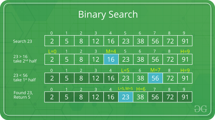
def binary_search(nums, target):
    """
    Searches for target in a sorted list by repeatedly halving the search space.

    After each step, we eliminate half the remaining elements.
    - 1000 elements: at most 10 steps  (2^10 = 1024)
    - 1 million elements: at most 20 steps  (2^20 = 1,048,576)
    - 1 billion elements: at most 30 steps  (2^30 = 1,073,741,824)

    Time complexity: O(log n)
    Space complexity: O(1)
    """
    left, right = 0, len(nums) - 1

    while left <= right:
        mid = (left + right) // 2  # find the middle index

        if nums[mid] == target:
            return mid              # found it
        elif nums[mid] < target:
            left = mid + 1          # target is in the right half
        else:
            right = mid - 1         # target is in the left half

    return -1  # not found

# Example
nums = [1, 3, 5, 7, 9, 11, 13, 15]
print(binary_search(nums, 7))   # 3  (index of 7)
print(binary_search(nums, 6))   # -1 (not found)
The key intuition: every time you double the input size, you only add one more step. That is the power of O(log n).
O(n) – Linear Time
The work grows directly in proportion to the input size. Double the input, double the work.
Real world analogy: Reading every page of a book to find a specific sentence. The longer the book, the longer it takes, directly proportionally.
def find_max(nums):
    """
    Finds the maximum value in an unsorted list.
    We have no choice but to look at every element at least once.

    Time complexity: O(n)  -- we visit each element exactly once
    Space complexity: O(1)  -- we only store the current max
    """
    max_val = float('-inf')  # start with negative infinity

    for num in nums:         # visit each element once -- this is the O(n) part
        if num > max_val:
            max_val = num

    return max_val

def linear_search(nums, target):
    """
    Searches for target by checking every element one by one.
    In the worst case, we check all n elements.

    Time complexity: O(n)
    Space complexity: O(1)
    """
    for i, num in enumerate(nums):
        if num == target:
            return i
    return -1
O(n log n) – Linearithmic Time
More than linear but much better than quadratic. This is the complexity of efficient sorting algorithms.
Intuition: Think of it as doing O(log n) work for each of the n elements. Or equivalently, splitting and merging the list O(log n) times, with each split/merge touching all n elements.
def merge_sort(nums):
    """
    Splits the list in half recursively, sorts each half,
    then merges the sorted halves back together.

    - Splitting happens log n times (we halve each time)
    - Each level of merging touches all n elements
    - Total: O(n log n)

    Time complexity: O(n log n)
    Space complexity: O(n)  -- we create new lists during merging
    """
    if len(nums) <= 1:
        return nums

    # Split into two halves
    mid = len(nums) // 2
    left = merge_sort(nums[:mid])   # sort left half
    right = merge_sort(nums[mid:])  # sort right half

    # Merge the two sorted halves
    return merge(left, right)

def merge(left, right):
    """Merges two sorted lists into one sorted list."""
    result = []
    i = j = 0

    while i < len(left) and j < len(right):
        if left[i] <= right[j]:
            result.append(left[i])
            i += 1
        else:
            result.append(right[j])
            j += 1

    # Append any remaining elements
    result.extend(left[i:])
    result.extend(right[j:])
    return result

# Example
nums = [5, 2, 8, 1, 9, 3]
print(merge_sort(nums))  # [1, 2, 3, 5, 8, 9]
Python’s built-in sort() and sorted() run in O(n log n). This is generally the best you can achieve for a comparison-based sort.
O(n^2) – Quadratic Time
The work grows with the square of the input size. Double the input, quadruple the work. This usually comes from nested loops where each loop runs n times.
Real world analogy: Comparing every person in a room to every other person. If there are 10 people, that is 100 comparisons. If there are 100 people, that is 10,000 comparisons.
def bubble_sort(nums):
    """
    Repeatedly steps through the list and swaps adjacent elements
    that are in the wrong order.

    For each of the n elements (outer loop), we potentially
    compare it against all other n elements (inner loop).

    Time complexity: O(n^2)
    Space complexity: O(1)  -- sorting is done in place
    """
    n = len(nums)

    for i in range(n):              # outer loop runs n times
        for j in range(n - i - 1): # inner loop runs roughly n times
            if nums[j] > nums[j + 1]:
                # swap adjacent elements
                nums[j], nums[j + 1] = nums[j + 1], nums[j]

    return nums

def has_duplicate_brute_force(nums):
    """
    Checks for duplicates by comparing every pair of elements.

    Time complexity: O(n^2)  -- nested loops, each running n times
    Space complexity: O(1)
    """
    n = len(nums)
    for i in range(n):
        for j in range(i + 1, n):  # compare nums[i] with every element after it
            if nums[i] == nums[j]:
                return True
    return False

def has_duplicate_efficient(nums):
    """
    The same problem solved with a hash set.

    Time complexity: O(n)   -- one pass through the list
    Space complexity: O(n)  -- the set can grow up to n elements
    """
    seen = set()
    for num in nums:
        if num in seen:  # O(1) lookup
            return True
        seen.add(num)
    return False
The duplicate detection example above is a perfect illustration of why complexity matters. The brute force O(n^2) solution and the O(n) solution both give the correct answer, but on a list of 1 million elements the O(n) solution will be roughly 1 million times faster.
O(2^n) – Exponential Time
The work doubles with each addition to the input. These algorithms become impractically slow very quickly.
When does this appear? Recursion that branches into two calls at each step, like a naive recursive Fibonacci or generating all subsets.
def fibonacci_naive(n):
    """
    Computes the nth Fibonacci number by recursively computing
    fibonacci(n-1) and fibonacci(n-2).

    The problem: each call spawns two more calls, and many
    subproblems are recomputed over and over.

    fibonacci(5) calls fibonacci(4) and fibonacci(3)
    fibonacci(4) calls fibonacci(3) and fibonacci(2)
    fibonacci(3) is computed multiple times -- wasteful

    Time complexity: O(2^n)  -- exponential, very slow for large n
    Space complexity: O(n)   -- call stack depth
    """
    if n <= 1:
        return n
    return fibonacci_naive(n - 1) + fibonacci_naive(n - 2)

def fibonacci_memo(n, memo={}):
    """
    Same computation but we store results we have already computed.
    This is called memoisation and is a core DP technique.

    Time complexity: O(n)  -- each value computed exactly once
    Space complexity: O(n)  -- memo dictionary stores n values
    """
    if n in memo:
        return memo[n]
    if n <= 1:
        return n
    memo[n] = fibonacci_memo(n - 1, memo) + fibonacci_memo(n - 2, memo)
    return memo[n]
O(n!) – Factorial Time
The slowest common complexity class. Generates all permutations of n elements.
def generate_permutations(nums):
    """
    Generates all possible orderings of a list.
    For n elements there are n! permutations.

    n=1: 1 permutation
    n=2: 2 permutations
    n=3: 6 permutations
    n=10: 3,628,800 permutations
    n=20: 2,432,902,008,176,640,000 permutations

    Time complexity: O(n!)
    Space complexity: O(n!)
    """
    if len(nums) == 0:
        return [[]]

    result = []
    for i, num in enumerate(nums):
        rest = nums[:i] + nums[i+1:]          # all elements except nums[i]
        for perm in generate_permutations(rest):  # permutations of the rest
            result.append([num] + perm)
    return result

print(generate_permutations([1, 2, 3]))
# [[1,2,3], [1,3,2], [2,1,3], [2,3,1], [3,1,2], [3,2,1]]
Comparing the Complexity Classes
Here is what the same input size looks like across different complexity classes. This table makes the differences visceral.
| n (input size) | O(1) | O(log n) | O(n) | O(n log n) | O(n^2) | O(2^n) |
|---|---|---|---|---|---|---|
| 10 | 1 | 3 | 10 | 33 | 100 | 1,024 |
| 100 | 1 | 7 | 100 | 664 | 10,000 | way too large |
| 1,000 | 1 | 10 | 1,000 | 9,966 | 1,000,000 | impossible |
| 1,000,000 | 1 | 20 | 1,000,000 | 19,931,568 | 10^12 | impossible |
Notice: O(n^2) with 1 million elements requires 1 trillion operations. At 10^9 operations per second, that is 1000 seconds. An O(n log n) solution does the same job in about 20 seconds. An O(n) solution does it in about 1 second.
How to Analyse Code Step by Step
Now that you know the complexity classes, here is a systematic process for analysing any piece of code.
Rule 1: A simple statement is O(1)
x = 5           # O(1)
y = x + 3       # O(1)
z = nums[i]     # O(1)
Rule 2: A loop that runs n times is O(n)
for i in range(n):   # runs n times
    print(i)         # O(1) work inside
# Total: O(n)
Rule 3: Nested loops multiply
for i in range(n):       # runs n times
    for j in range(n):   # runs n times for each i
        print(i, j)      # O(1) work inside
# Total: O(n * n) = O(n^2)
Rule 4: Sequential blocks add, and we keep only the dominant term
for i in range(n):   # O(n)
    print(i)

for i in range(n):   # O(n)
    for j in range(n):
        print(i, j)  # O(n^2)

# Total: O(n) + O(n^2) = O(n^2)  -- we drop the lower order term
Rule 5: If the loop variable halves each time, it is O(log n)
i = n
while i > 0:
    print(i)
    i = i // 2   # i halves each iteration
# Total: O(log n)
Putting it all together – a real example:
def example(nums):
    """
    Let's analyse this function step by step.
    nums has n elements.
    """

    # Step 1: Find the maximum -- one pass through the list
    max_val = float('-inf')          # O(1)
    for num in nums:                 # loop runs n times
        max_val = max(max_val, num)  # O(1) work
    # This block: O(n)

    # Step 2: Find all pairs that sum to max_val
    result = []                      # O(1)
    for i in range(len(nums)):       # loop runs n times
        for j in range(i+1, len(nums)):  # loop runs up to n times
            if nums[i] + nums[j] == max_val:  # O(1)
                result.append((nums[i], nums[j]))  # O(1)
    # This block: O(n^2)

    return result

# Total: O(n) + O(n^2) = O(n^2)
# The O(n^2) block dominates, so the overall complexity is O(n^2)
Space Complexity
Space complexity measures how much extra memory an algorithm uses relative to the input size. The rules are similar to time complexity.
Note: we do not count the input itself – we count the additional memory the algorithm allocates.
def sum_list(nums):
    """
    Adds up all elements. Only stores the running total.

    Time complexity: O(n)
    Space complexity: O(1)  -- only one extra variable regardless of input size
    """
    total = 0
    for num in nums:
        total += num
    return total

def double_all(nums):
    """
    Creates a new list with each element doubled.

    Time complexity: O(n)
    Space complexity: O(n)  -- the new list grows with the input
    """
    result = []
    for num in nums:
        result.append(num * 2)
    return result

def two_sum(nums, target):
    """
    Finds two indices that add up to target using a hash map.

    Time complexity: O(n)   -- one pass through nums
    Space complexity: O(n)  -- the seen dictionary can hold up to n entries
    """
    seen = {}  # maps value to its index
    for i, num in enumerate(nums):
        complement = target - num
        if complement in seen:
            return [seen[complement], i]
        seen[num] = i
    return []
Space complexity of recursion: Each recursive call adds a frame to the call stack. If a function calls itself n times deep, the space complexity is at least O(n).
def factorial(n):
    """
    Computes n! recursively.

    Time complexity: O(n)  -- n recursive calls
    Space complexity: O(n) -- n frames on the call stack at maximum depth
    """
    if n == 0:
        return 1
    return n * factorial(n - 1)
Common Misconceptions
Misconception 1: Faster computer means better algorithm
A faster computer makes every algorithm faster by a constant factor. It does not change the complexity class. An O(n^2) algorithm on a computer 1000x faster is still O(n^2) – it will still be slower than an O(n) algorithm at large enough inputs.
Misconception 2: O(n^2) is always bad
For small inputs, an O(n^2) algorithm can be perfectly fine. If you know n will never exceed 100, the difference between O(n) and O(n^2) is negligible. Complexity analysis matters most at scale.
Misconception 3: The best complexity is always the goal
Sometimes an O(n log n) solution is harder to write and maintain than an O(n^2) solution, and the input is small enough that it does not matter. Always consider the constraints. For n <= 100, almost anything works. For n >= 10^6, you need to think carefully.
Misconception 4: Big O is the whole story
Two algorithms can both be O(n log n) but one can be twice as fast in practice because of constant factors, cache behaviour, or simpler code. Big O tells you the shape of growth, not the exact performance.
Misconception 5: Space and time are independent
Often you trade one for the other. The duplicate detection example earlier used O(n) space to get O(n) time instead of O(1) space with O(n^2) time. This trade-off comes up constantly.
Complexity of Python Built-ins (Reference)
Now that you understand complexity, the table from the Python Refresher blog will make complete sense.
| Operation | Time Complexity |
|---|---|
list[i] | O(1) |
list.append(x) | O(1) amortised |
list.insert(i, x) | O(n) |
x in list | O(n) |
x in dict | O(1) average |
x in set | O(1) average |
list.sort() | O(n log n) |
len(list) | O(1) |
dict[key] | O(1) average |
heapq.heappush | O(log n) |
heapq.heappop | O(log n) |
Practice Problems
Work through these in order. For each one, state the time and space complexity of your solution before looking at the answer.
Problem 1 – Count the Steps (Easy)
What is the time complexity of the following function? Explain your reasoning.
def mystery(n):
    count = 0
    i = 1
    while i < n:
        count += 1
        i *= 2
    return count
Think about it: What does i *= 2 do to i on each iteration? How many times can you double i before it reaches n?
Answer:
The variable i starts at 1 and doubles each iteration: 1, 2, 4, 8, 16 ...
It reaches n after log2(n) steps.
Time complexity: O(log n)
Space complexity: O(1)
Problem 2 – Two Sum (Easy)
Given a list of integers and a target, return the indices of two numbers that add up to the target. Each input has exactly one solution.
# Example
nums = [2, 7, 11, 15]
target = 9
# Output: [0, 1]  because nums[0] + nums[1] = 2 + 7 = 9
Approach 1 – Brute Force:
def two_sum_brute(nums, target):
    """
    Check every pair of elements.

    Time complexity: O(n^2)  -- nested loops
    Space complexity: O(1)   -- no extra data structures
    """
    n = len(nums)
    for i in range(n):
        for j in range(i + 1, n):       # j starts after i to avoid using same element twice
            if nums[i] + nums[j] == target:
                return [i, j]
    return []
Approach 2 – Hash Map:
def two_sum_optimal(nums, target):
    """
    For each number, check if its complement (target - num) has been seen before.
    Store each number and its index in a dictionary as we go.

    Time complexity: O(n)   -- single pass through the list
    Space complexity: O(n)  -- dictionary can hold up to n entries
    """
    seen = {}  # maps number to its index

    for i, num in enumerate(nums):
        complement = target - num       # what do we need to pair with num?

        if complement in seen:          # O(1) lookup -- have we seen the complement?
            return [seen[complement], i]

        seen[num] = i                   # store current number and its index

    return []

# Test
print(two_sum_optimal([2, 7, 11, 15], 9))   # [0, 1]
print(two_sum_optimal([3, 2, 4], 6))         # [1, 2]
Problem 3 – Count Unique Values (Easy)
Given a sorted list, count the number of unique values without using a set.
# Example
nums = [1, 1, 2, 3, 3, 4, 4, 4, 5]
# Output: 5  (values 1, 2, 3, 4, 5)
def count_unique(nums):
    """
    Since the list is sorted, duplicates are adjacent.
    We just count how many times the value changes.

    Time complexity: O(n)   -- single pass
    Space complexity: O(1)  -- only store the count and last seen value
    """
    if not nums:
        return 0

    count = 1                          # first element is always unique

    for i in range(1, len(nums)):
        if nums[i] != nums[i - 1]:    # value changed -- new unique element
            count += 1

    return count

print(count_unique([1, 1, 2, 3, 3, 4, 4, 4, 5]))  # 5
print(count_unique([]))                              # 0
print(count_unique([7]))                             # 1
Problem 4 – Analyse This Function (Medium)
What is the time and space complexity of the following function?
def process(nums):
    n = len(nums)
    result = []

    for i in range(n):
        total = 0
        for j in range(i, n):
            total += nums[j]
            result.append(total)

    return result
Answer:
Outer loop runs n times.
Inner loop runs n - i times for each i, which on average is n/2 times.
Total iterations: roughly n * n/2 = n^2/2 operations.
We drop the constant: O(n^2)

For space: the result list. How many elements does it hold?
i=0: n elements appended
i=1: n-1 elements appended
...
i=n-1: 1 element appended
Total: n + (n-1) + ... + 1 = n(n+1)/2 elements

Space complexity: O(n^2)
Summary
| Complexity | Name | Example | How it grows |
|---|---|---|---|
| O(1) | Constant | Array index access, dict lookup | Does not grow |
| O(log n) | Logarithmic | Binary search | Grows by 1 step when input doubles |
| O(n) | Linear | Linear search, single loop | Doubles when input doubles |
| O(n log n) | Linearithmic | Merge sort, heapsort | Slightly more than linear |
| O(n^2) | Quadratic | Bubble sort, nested loops | Quadruples when input doubles |
| O(2^n) | Exponential | Naive recursion, subsets | Doubles with each new element |
| O(n!) | Factorial | Permutations | Grows faster than any of the above |
Key Takeaways
- Complexity analysis describes how an algorithm scales, independent of hardware or language.
- Big O notation captures the dominant term and drops constants. O(3n + 5) is O(n).
- Nested loops usually mean O(n^2). A loop that halves its range each time is O(log n).
- Space complexity measures extra memory used, not the input itself.
- You often trade space for time. Using a hash map turns an O(n^2) problem into O(n) at the cost of O(n) space.
- Complexity is most important at scale. For tiny inputs, any solution works.
- Always state the time and space complexity of every solution you write. Make it a habit from day one.
Next Steps
- Next blog: [Arrays] – the first data structure, covered in full depth, with all operations and patterns
- Reference: Codeverra DSA Sheet