Arrays
Table of Contents
- What You Will Learn in This Blog
- How Data is Stored in Computer Memory
- What is an Array
- Arrays in Python
- Referential Arrays vs Value Arrays
- Dynamic Arrays – How Python Lists Grow
- Time and Space Complexity of Array Operations
- Two-Dimensional Arrays
- Patterns and Techniques
- Summary
- Key Takeaways
- Practice Problems
- Next Steps
What You Will Learn in This Blog
- How data is stored in computer memory and why it matters
- What an array is and how it uses contiguous memory
- How Python represents arrays – lists, the array module, and NumPy
- The difference between referential arrays and value arrays
- How dynamic arrays work and how Python lists resize themselves
- Time and space complexity of every common array operation
- Three core patterns that come from arrays: Two Pointers, Sliding Window, and Prefix Sum
- Solved LeetCode problems for each pattern
- A practice problem table for further study
How Data is Stored in Computer Memory
Before we talk about arrays, we need to understand the environment arrays live in – computer memory.
When your program runs, it gets access to RAM (Random Access Memory). You can think of RAM as a very long row of small storage boxes. Each box:
- Holds exactly one byte (8 bits) of data
- Has a unique address – a number that identifies its position

When you store a value, the computer places it at some address in memory. When you want to read it back, the computer goes directly to that address. This direct access by address is extremely fast – it is O(1) regardless of how large the memory is or where in memory the value lives.
Here is the key insight: if you know the starting address and the size of each element, you can calculate the address of any element instantly using simple arithmetic.
address of element at index i = starting_address + (i * size_of_each_element)
This formula is why arrays are so powerful. And it only works because of one critical requirement: the elements must be stored in a contiguous block of memory – one right after the other, with no gaps.
What is an Array
An array is a collection of elements stored in contiguous memory locations, where every element is of the same size.
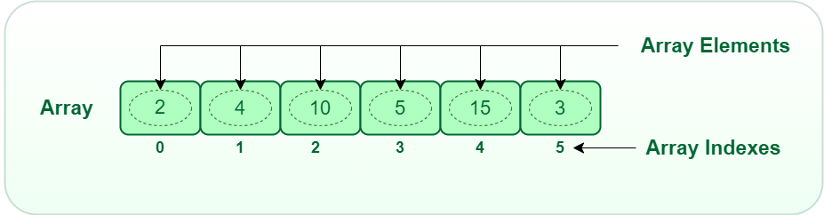
Consider an array of integers: [10, 20, 30, 40, 50]
If each integer takes 4 bytes and the array starts at memory address 1000, here is how it looks in memory:
| Index | Value | Memory Address |
|---|---|---|
| 0 | 10 | 1000 |
| 1 | 20 | 1004 |
| 2 | 30 | 1008 |
| 3 | 40 | 1012 |
| 4 | 50 | 1016 |
To access arr[3], the computer calculates:
address = 1000 + (3 * 4) = 1012
It goes directly to address 1012 and reads the value. This is one arithmetic operation and one memory read – O(1) regardless of array size. It does not scan from the beginning. It jumps straight there.
This is the fundamental reason array access by index is O(1), and it is one of the most important ideas in all of computer science.
Arrays in Python
Python gives you three ways to work with arrays, and they are quite different from each other.
Python Lists
Python’s built-in list is what you will use for almost everything in this guide. It is a dynamic array – it can grow and shrink as needed.
# Creating a list
nums = [10, 20, 30, 40, 50]

# Accessing by index -- O(1)
print(nums[0])   # 10
print(nums[2])   # 30
print(nums[-1])  # 50  (negative index counts from the end)

# Modifying an element -- O(1)
nums[1] = 99
print(nums)  # [10, 99, 30, 40, 50]

# Length -- O(1)
print(len(nums))  # 5
Python lists are incredibly flexible but they come with an important caveat that we will cover shortly – they do not store values directly. They store references to objects.
The array Module
Python’s built-in array module gives you a true value array – it stores actual values of a fixed type, not references. This uses less memory than a list when you have large amounts of numeric data.
import array

# Create an array of signed integers ('i' is the type code for int)
nums = array.array('i', [10, 20, 30, 40, 50])

print(nums[0])   # 10
print(nums[2])   # 30

# Common type codes
# 'i' -- signed int (4 bytes)
# 'f' -- float (4 bytes)
# 'd' -- double / float64 (8 bytes)
# 'b' -- signed char / int8 (1 byte)
In DSA problems you will almost never need the array module – Python lists are used universally. But it is worth knowing it exists and why it is different.
NumPy Arrays
NumPy is a third-party library built for numerical computing. NumPy arrays are true value arrays and support fast vectorised operations on large datasets.
import numpy as np

# Create a NumPy array
nums = np.array([10, 20, 30, 40, 50])

print(nums[0])    # 10
print(nums.dtype) # int64  -- all elements are the same type

# Vectorised operations -- applied to every element at once
print(nums * 2)   # [20 40 60 80 100]
print(nums + 10)  # [20 30 40 50 60]

# 2D arrays (matrices)
matrix = np.array([[1, 2, 3],
                   [4, 5, 6],
                   [7, 8, 9]])
print(matrix[1][2])  # 6  -- row 1, column 2
For DSA problems, NumPy is rarely needed. It matters more in data science and machine learning. We mention it here for completeness.
Comparison of the Three
| Feature | Python list | array module | NumPy array |
|---|---|---|---|
| Stores | References to objects | Actual values | Actual values |
| Element types | Mixed (any type) | Fixed type | Fixed type |
| Memory usage | Higher | Lower | Lower |
| Speed (numeric ops) | Slower | Faster | Fastest |
| Flexibility | Highest | Medium | Medium |
| Use in DSA | Always | Rarely | Rarely |
Referential Arrays vs Value Arrays
This is one of the most important things to understand about Python lists, and it is something that surprises many beginners.
In languages like C, an array of integers stores the actual integer values side by side in memory. Python lists do not work this way.
A Python list stores references (memory addresses pointing to objects), not the values themselves. Each element in the list is a pointer to a Python object somewhere else in memory.
nums = [10, 20, 30]

# What Python actually stores in the list:
# [ pointer_to_10, pointer_to_20, pointer_to_30 ]
# Each pointer is 8 bytes on a 64-bit system
# The actual integer objects live elsewhere in memory
This has several consequences:
1. A Python list can hold mixed types because it stores references, not values
mixed = [42, "hello", 3.14, True, [1, 2, 3]]
# All valid -- each element is just a pointer to a different type of object
2. Assignment copies the reference, not the value
a = [1, 2, 3]
b = a           # b points to the SAME list as a, not a copy

b[0] = 99
print(a)        # [99, 2, 3]  -- a is also changed!
print(b)        # [99, 2, 3]

# To make a true copy, use slicing or list()
c = a[:]        # or list(a) or a.copy()
c[0] = 0
print(a)        # [99, 2, 3]  -- a is unchanged
print(c)        # [0, 2, 3]
3. Equality vs identity
a = [1, 2, 3]
b = [1, 2, 3]
c = a

print(a == b)   # True  -- same values
print(a is b)   # False -- different objects in memory
print(a is c)   # True  -- same object in memory
Understanding this distinction prevents many subtle bugs, especially when you pass lists to functions or try to make copies.
Dynamic Arrays – How Python Lists Grow
A regular array has a fixed size – you declare it with a certain capacity and it cannot grow. Python lists, however, can grow dynamically. How does this work?
Under the hood, Python allocates more memory than the list currently needs. When the list fills up, Python allocates a new, larger block of memory, copies everything over, and releases the old block.

Here is the key detail: Python does not just add one slot at a time. It roughly doubles the capacity each time. This is called the doubling strategy.
Let us trace through what happens as you append elements:
| Append call | List size | Allocated capacity | Action |
|---|---|---|---|
| Start | 0 | 0 | – |
| append(1) | 1 | 4 | Allocate space for 4 |
| append(2) | 2 | 4 | No resize needed |
| append(3) | 3 | 4 | No resize needed |
| append(4) | 4 | 4 | No resize needed |
| append(5) | 5 | 8 | Resize: copy 4 elements to new block of 8 |
| append(6) | 6 | 8 | No resize needed |
| append(7) | 7 | 8 | No resize needed |
| append(8) | 8 | 8 | No resize needed |
| append(9) | 9 | 16 | Resize: copy 8 elements to new block of 16 |
Most appends are O(1). Occasionally one append triggers a resize, which takes O(n) to copy everything. But because resizes happen less and less frequently as the list grows, the amortised cost per append is still O(1).
Amortised means: averaged over a long sequence of operations. A single append might take O(n), but if you do n appends total, the total work is O(n), so each append costs O(1) on average.
import sys

# You can see Python allocating extra capacity
nums = []
for i in range(10):
    nums.append(i)
    # sys.getsizeof gives the memory size of the list object in bytes
    print(f"Length: {len(nums)}, Memory: {sys.getsizeof(nums)} bytes")

# Output (approximate, varies by Python version):
# Length: 1, Memory: 88 bytes
# Length: 2, Memory: 88 bytes
# Length: 3, Memory: 88 bytes
# Length: 4, Memory: 88 bytes
# Length: 5, Memory: 120 bytes  <-- resize happened
# Length: 6, Memory: 120 bytes
# ...
Time and Space Complexity of Array Operations
Now that you understand how arrays work internally, the complexity of each operation should make intuitive sense.
| Operation | Code | Time Complexity | Why |
|---|---|---|---|
| Access by index | nums[i] | O(1) | Direct address calculation |
| Update by index | nums[i] = x | O(1) | Direct address calculation |
| Append to end | nums.append(x) | O(1) amortised | Occasional O(n) resize |
| Pop from end | nums.pop() | O(1) | No shifting needed |
| Insert at index i | nums.insert(i, x) | O(n) | Must shift all elements after i |
| Delete at index i | del nums[i] | O(n) | Must shift all elements after i |
| Search for value | x in nums | O(n) | Must scan the entire list |
| Get length | len(nums) | O(1) | Stored as a property |
Slice [i:j] | nums[i:j] | O(k) | k = j - i, copies k elements |
| Concatenate | a + b | O(n + m) | Copies both lists |
| Sort | nums.sort() | O(n log n) | Timsort |
| Reverse | nums.reverse() | O(n) | Visits every element once |
| Copy | nums.copy() | O(n) | Copies every element |
The most important thing to remember: inserting or deleting at the beginning or middle of a list is O(n) because every element after that position must shift. This is the main weakness of arrays compared to linked lists.
Two-Dimensional Arrays
A 2D array is an array of arrays. It is used to represent grids, matrices, and boards.
# Creating a 2D list (3 rows, 4 columns)
matrix = [
    [1,  2,  3,  4],
    [5,  6,  7,  8],
    [9, 10, 11, 12]
]

# Accessing an element -- O(1)
print(matrix[1][2])   # 7  -- row 1, column 2
print(matrix[0][0])   # 1  -- top left
print(matrix[2][3])   # 12 -- bottom right

# Iterating over a 2D array
for row in matrix:
    for val in row:
        print(val, end=" ")
    print()

# Creating an n x m grid filled with zeros
n, m = 3, 4
grid = [[0] * m for _ in range(n)]
print(grid)
# [[0, 0, 0, 0],
#  [0, 0, 0, 0],
#  [0, 0, 0, 0]]

# WARNING -- do NOT do this
bad_grid = [[0] * m] * n
# This creates n references to the SAME row
# Modifying one row modifies all of them
bad_grid[0][0] = 99
print(bad_grid)
# [[99, 0, 0, 0],
#  [99, 0, 0, 0],   <-- all rows changed!
#  [99, 0, 0, 0]]
Patterns and Techniques
Now we get to the techniques that make arrays so powerful in problem solving. Each of these patterns comes directly from the properties of arrays – indexed access, contiguity, and ordering.
Pattern 1 – Two Pointers
The core idea: Use two index variables that move through the array, usually from opposite ends toward the middle or in the same direction at different speeds. This turns many O(n^2) problems into O(n).
When to use it:
- The array is sorted (or you can sort it)
- You are looking for a pair of elements that satisfy some condition
- You need to remove or partition elements in place

The template:
left, right = 0, len(nums) - 1

while left < right:
    # use nums[left] and nums[right]
    # move left forward, right backward, or both
    # based on the condition of the problem
    if some_condition:
        left += 1
    elif some_other_condition:
        right -= 1
    else:
        left += 1
        right -= 1
Solved Problem – Valid Palindrome
LeetCode 125 – Valid Palindrome
Problem: A phrase is a palindrome if, after converting all uppercase letters to lowercase and removing all non-alphanumeric characters, it reads the same forward and backward. Given a string s, return True if it is a palindrome, otherwise return False.
Input:  s = "A man, a plan, a canal: Panama"
Output: True

Input:  s = "race a car"
Output: False
Thinking through it:
A brute force approach would be to clean the string first, then check if it equals its reverse. That works in O(n) time and O(n) space (for the cleaned string).
But we can do better on space. Instead of building a new string, use two pointers – one at the start, one at the end. Skip non-alphanumeric characters and compare characters as you go. If they ever differ, it is not a palindrome.
def is_palindrome(s: str) -> bool:
    """
    Uses two pointers starting from both ends, moving inward.
    Skip any character that is not alphanumeric.
    Compare the characters at both pointers -- if they ever differ, return False.

    Time complexity:  O(n) -- each character is visited at most once
    Space complexity: O(1) -- no extra data structures, just two index variables
    """
    left, right = 0, len(s) - 1

    while left < right:

        # Move left pointer forward past non-alphanumeric characters
        while left < right and not s[left].isalnum():
            left += 1

        # Move right pointer backward past non-alphanumeric characters
        while left < right and not s[right].isalnum():
            right -= 1

        # Compare characters (case insensitive)
        if s[left].lower() != s[right].lower():
            return False  # mismatch -- not a palindrome

        # Both matched, move both pointers inward
        left += 1
        right -= 1

    return True  # all characters matched

# Test cases
print(is_palindrome("A man, a plan, a canal: Panama"))  # True
print(is_palindrome("race a car"))                       # False
print(is_palindrome(" "))                                # True (empty after cleaning)
Solved Problem – Container With Most Water
LeetCode 11 – Container With Most Water
Problem: You are given an integer array height of length n. There are n vertical lines drawn such that the two endpoints of the ith line are (i, 0) and (i, height[i]). Find two lines that together with the x-axis form a container that holds the most water. Return the maximum amount of water a container can store.
Input:  height = [1, 8, 6, 2, 5, 4, 8, 3, 7]
Output: 49
Thinking through it:
The brute force is to check every pair of lines – O(n^2). Can we do better?
The water between lines at index left and right is:
water = min(height[left], height[right]) * (right - left)
Start with the widest possible container (left = 0, right = n-1). To try to find more water, we need to increase the height. Moving the pointer at the taller side inward cannot help – the height is still limited by the shorter side and the width decreases. So we always move the pointer at the shorter side inward, hoping to find a taller line.
def max_area(height: list) -> int:
    """
    Start with the widest container. At each step, move the pointer
    at the shorter side inward -- this is the only move that could
    possibly find more water.

    Time complexity:  O(n) -- each element is visited at most once
    Space complexity: O(1) -- only two pointers and a max variable
    """
    left, right = 0, len(height) - 1
    max_water = 0

    while left < right:
        # Calculate water in current container
        width = right - left
        h = min(height[left], height[right])
        current_water = width * h

        # Update maximum
        max_water = max(max_water, current_water)

        # Move the pointer at the shorter side inward
        if height[left] < height[right]:
            left += 1
        else:
            right -= 1

    return max_water

# Test
print(max_area([1, 8, 6, 2, 5, 4, 8, 3, 7]))  # 49
print(max_area([1, 1]))                          # 1
Pattern 2 – Sliding Window
The core idea: Maintain a window (a contiguous subarray) that slides across the array. Instead of recomputing the result from scratch for each window position, you add the new element entering the window and remove the element leaving it. This turns many O(n^2) subarray problems into O(n).
When to use it:
- You need to find a subarray or substring that satisfies some condition
- The condition involves something about a contiguous range (sum, count, unique elements)
- The problem involves “maximum”, “minimum”, or “longest” subarray with a constraint

Two types of sliding window:
Fixed size window – the window size k is given:
# Template: fixed window of size k
def fixed_window(nums, k):
    # Build the first window
    window_sum = sum(nums[:k])
    result = window_sum

    # Slide the window: add right element, remove left element
    for i in range(k, len(nums)):
        window_sum += nums[i]        # add element entering window
        window_sum -= nums[i - k]    # remove element leaving window
        result = max(result, window_sum)

    return result
Variable size window – find the longest/shortest window satisfying a condition:
# Template: variable window
def variable_window(nums):
    left = 0
    result = 0

    for right in range(len(nums)):
        # Expand: include nums[right] in the window

        while # window condition is violated:
            # Shrink: remove nums[left] from the window
            left += 1

        # Window is now valid -- update result
        result = max(result, right - left + 1)

    return result
Solved Problem – Best Time to Buy and Sell Stock
LeetCode 121 – Best Time to Buy and Sell Stock
Problem: You are given an array prices where prices[i] is the price of a stock on day i. You want to buy on one day and sell on a later day to maximise profit. Return the maximum profit. If no profit is possible, return 0.
Input:  prices = [7, 1, 5, 3, 6, 4]
Output: 5  (buy on day 1 at price 1, sell on day 4 at price 6)

Input:  prices = [7, 6, 4, 3, 1]
Output: 0  (prices only go down, no profit possible)
Thinking through it:
The brute force checks every pair of days – O(n^2). The key observation is: the best profit on any given day is price[today] - minimum_price_seen_so_far. So we only need one pass, tracking the minimum price seen so far and the maximum profit seen so far.
This is a sliding window in spirit – the window is from the minimum price day to the current day.
def max_profit(prices: list) -> int:
    """
    Track the minimum price seen so far.
    At each day, compute the profit if we sold today.
    Update the maximum profit if this is better.

    Time complexity:  O(n) -- single pass through prices
    Space complexity: O(1) -- only two variables
    """
    min_price = float('inf')  # smallest price seen so far
    max_profit = 0            # best profit seen so far

    for price in prices:
        if price < min_price:
            min_price = price            # found a better day to buy
        else:
            profit = price - min_price   # profit if we sell today
            max_profit = max(max_profit, profit)

    return max_profit

# Test
print(max_profit([7, 1, 5, 3, 6, 4]))  # 5
print(max_profit([7, 6, 4, 3, 1]))      # 0
print(max_profit([2, 4, 1]))            # 2
Solved Problem – Maximum Average Subarray I
LeetCode 643 – Maximum Average Subarray I
Problem: You are given an integer array nums consisting of n elements, and an integer k. Find a contiguous subarray of length exactly k that has the maximum average value and return this value.
Input:  nums = [1, 12, -5, -6, 50, 3], k = 4
Output: 12.75  (subarray [12, -5, -6, 50], average = 51/4 = 12.75)
Thinking through it:
This is a fixed-size sliding window. Build the first window of size k, then slide it across, adding the new element and removing the old one. Track the maximum sum seen.
def find_max_average(nums: list, k: int) -> float:
    """
    Fixed sliding window of size k.
    Compute the sum of the first window, then slide it across
    by adding the incoming element and removing the outgoing one.

    Time complexity:  O(n) -- one pass after the initial window
    Space complexity: O(1) -- only store the current and max sum
    """
    # Build the first window
    window_sum = sum(nums[:k])    # O(k) but k <= n so overall still O(n)
    max_sum = window_sum

    # Slide the window from position k to end
    for i in range(k, len(nums)):
        window_sum += nums[i]       # element entering the window
        window_sum -= nums[i - k]   # element leaving the window
        max_sum = max(max_sum, window_sum)

    return max_sum / k

# Test
print(find_max_average([1, 12, -5, -6, 50, 3], 4))  # 12.75
print(find_max_average([5], 1))                       # 5.0
Pattern 3 – Prefix Sum
The core idea: Precompute a running total of the array so that the sum of any subarray nums[i:j] can be computed in O(1) instead of O(n).
The formula:
prefix[0] = 0
prefix[i] = nums[0] + nums[1] + ... + nums[i-1]

sum of nums[left..right] = prefix[right + 1] - prefix[left]
When to use it:
- Multiple queries asking for the sum of a subarray
- Problems involving subarray sums equal to a target
- Any problem where you need to quickly compute the sum of a range

The template:
def build_prefix(nums):
    n = len(nums)
    prefix = [0] * (n + 1)   # prefix[0] = 0 by convention
    for i in range(n):
        prefix[i + 1] = prefix[i] + nums[i]
    return prefix

# Query: sum of nums[left..right] inclusive
def range_sum(prefix, left, right):
    return prefix[right + 1] - prefix[left]
Solved Problem – Range Sum Query - Immutable
LeetCode 303 – Range Sum Query - Immutable
Problem: Given an integer array nums, handle multiple queries of the form: calculate the sum of elements between indices left and right inclusive.
Input:  nums = [-2, 0, 3, -5, 2, -1]
        sumRange(0, 2) --> 1   (-2 + 0 + 3)
        sumRange(2, 5) --> -1  (3 + -5 + 2 + -1)
        sumRange(0, 5) --> -3  (-2 + 0 + 3 + -5 + 2 + -1)
Thinking through it:
If we compute the sum naively for each query, each query costs O(n) and with q queries the total is O(n * q). With a prefix sum array, each query costs O(1) after an O(n) preprocessing step.
class NumArray:
    """
    Precompute prefix sums once at initialisation.
    Answer each range query in O(1).

    Time complexity:
        __init__: O(n) -- build the prefix sum array
        sumRange:  O(1) -- subtract two prefix values

    Space complexity: O(n) -- the prefix sum array
    """

    def __init__(self, nums: list):
        n = len(nums)
        # prefix[i] = sum of nums[0..i-1]
        # prefix[0] = 0  (sum of empty prefix)
        self.prefix = [0] * (n + 1)

        for i in range(n):
            self.prefix[i + 1] = self.prefix[i] + nums[i]

    def sumRange(self, left: int, right: int) -> int:
        # sum of nums[left..right]
        # = (sum of nums[0..right]) - (sum of nums[0..left-1])
        # = prefix[right + 1] - prefix[left]
        return self.prefix[right + 1] - self.prefix[left]

# Test
obj = NumArray([-2, 0, 3, -5, 2, -1])
print(obj.sumRange(0, 2))  # 1
print(obj.sumRange(2, 5))  # -1
print(obj.sumRange(0, 5))  # -3
Solved Problem – Subarray Sum Equals K
LeetCode 560 – Subarray Sum Equals K
Problem: Given an array of integers nums and an integer k, return the total number of subarrays whose sum equals k.
Input:  nums = [1, 1, 1], k = 2
Output: 2

Input:  nums = [1, 2, 3], k = 3
Output: 2
Thinking through it:
The brute force is O(n^2): try every subarray. Can we do better?
The sum of subarray nums[i..j] equals prefix[j+1] - prefix[i]. We want this to equal k, which means we want prefix[i] = prefix[j+1] - k.
So as we compute the prefix sum, we check: have we seen a prefix sum equal to current_prefix - k before? If yes, we have found subarrays that sum to k. We use a hash map to track prefix sums seen so far.
def subarray_sum(nums: list, k: int) -> int:
    """
    As we build the prefix sum, we ask at each position j:
    how many previous prefix sums equal (current_prefix - k)?
    Each such prefix sum corresponds to a valid subarray ending at j.

    Time complexity:  O(n) -- single pass
    Space complexity: O(n) -- hash map stores up to n prefix sums
    """
    count = 0
    prefix_sum = 0
    # Maps prefix_sum value to how many times we have seen it
    seen = {0: 1}   # prefix sum of 0 exists once before we start

    for num in nums:
        prefix_sum += num                       # update running prefix sum

        # How many previous positions had prefix sum = prefix_sum - k?
        # Each one gives a subarray ending here that sums to k
        complement = prefix_sum - k
        count += seen.get(complement, 0)        # O(1) lookup

        # Record this prefix sum
        seen[prefix_sum] = seen.get(prefix_sum, 0) + 1

    return count

# Test
print(subarray_sum([1, 1, 1], 2))  # 2
print(subarray_sum([1, 2, 3], 3))  # 2
print(subarray_sum([1, -1, 1], 0)) # 3
Summary
What We Covered
| Topic | Key Point |
|---|---|
| Computer memory | RAM is a sequence of addressed bytes. Knowing the start address and element size lets you reach any index in O(1) |
| Arrays | Contiguous memory block. Fixed element size. O(1) access by index |
| Python lists | Dynamic array. Stores references, not values. Resizes by doubling |
| array module | True value array. Fixed type. Less memory than a list |
| NumPy arrays | High-performance value array. Used in data science, rarely in DSA |
| Referential arrays | Python lists store pointers. Assignment copies the pointer, not the value |
| Dynamic arrays | Extra capacity allocated. Amortised O(1) append. Occasional O(n) resize |
| 2D arrays | Array of arrays. Create with list comprehension, not [[0]*m]*n |
Operation Complexity at a Glance
| Operation | Complexity |
|---|---|
| Access / update by index | O(1) |
| Append to end | O(1) amortised |
| Pop from end | O(1) |
| Insert at position i | O(n) |
| Delete at position i | O(n) |
| Search (unsorted) | O(n) |
| Sort | O(n log n) |
| Slice [i:j] | O(k) where k = j - i |
Patterns Introduced
| Pattern | Core idea | Time complexity gain | Use when |
|---|---|---|---|
| Two Pointers | Two indices moving through the array | O(n^2) to O(n) | Pair problems, sorted arrays, in-place operations |
| Sliding Window | Maintain a window, add right, remove left | O(n^2) to O(n) | Subarray/substring with a constraint |
| Prefix Sum | Precompute cumulative sums | O(n) per query to O(1) | Range sum queries, subarray sum problems |
Key Takeaways
- Array access is O(1) because of contiguous memory and direct address calculation. This is the most fundamental property of arrays.
- Python lists are dynamic and store references, not values. Assigning a list to another variable does not copy it.
- Insert and delete in the middle of an array are O(n) because elements must shift. This is the main weakness of arrays.
- The doubling strategy gives Python lists amortised O(1) append.
- Two Pointers, Sliding Window, and Prefix Sum are patterns that exploit the indexed, ordered nature of arrays to solve problems efficiently.
- Always create 2D arrays with
[[0]*m for _ in range(n)], not[[0]*m]*n.
Practice Problems
Work through these on your own. For each problem, think about which pattern applies before writing any code.
| Problem | Link | Difficulty | Pattern |
|---|---|---|---|
| Two Sum | LC 1 | Easy | Hash Map |
| Remove Duplicates from Sorted Array | LC 26 | Easy | Two Pointers |
| Move Zeroes | LC 283 | Easy | Two Pointers |
| Squares of a Sorted Array | LC 977 | Easy | Two Pointers |
| Maximum Subarray | LC 53 | Medium | Sliding Window / Kadane’s |
| Minimum Size Subarray Sum | LC 209 | Medium | Sliding Window |
| 3Sum | LC 15 | Medium | Two Pointers |
| Product of Array Except Self | LC 238 | Medium | Prefix Sum |
| Contiguous Array | LC 525 | Medium | Prefix Sum + Hash Map |
| Trapping Rain Water | LC 42 | Hard | Two Pointers / Prefix Sum |
Next Steps
- Next blog: [Strings] – strings are closely related to arrays and share several of the same patterns
- Reference: Codeverra DSA Sheet